Best practices for beginning to visualize your customers through bar plots, heat maps, line plots, and histograms

Congratulations! If you’re here to learn about data and visualizing your customers, it means you’ve already found your first customers - a big step on its own! Whether your product is a game, a new method of transportation, or the next great innovation in spray cheese, it’s now critical to understand who your customers are and how to make the best product for them - all while continuing to grow. Today we’ll go over four simple starting points we use at Datawisp for beginning to understand who is interacting with your product.

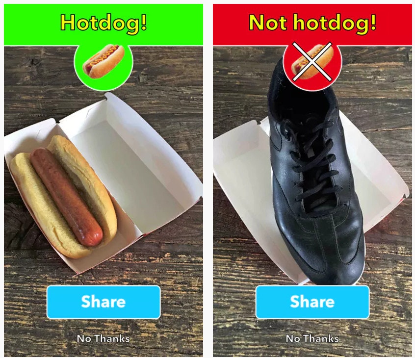
Let’s put ourselves in the shoes of a tech startup. We’ve just launched v1.0 of our revolutionary new app “Not Hotdog”, which uses the camera to identify whether the food in question is or is not a hot dog. Naturally, downloads are going through the roof and with users, comes data to analyze.

Who are our customers? - Bar Plot

Logically, the first question we might want to ask is “Who are our customers?”. The app store can collect all the data we need for this, and we don’t need any machine learning or incredibly technical data science to start finding answers.

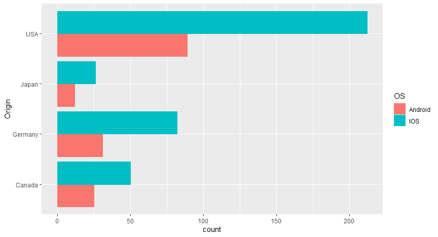
A fairly simple bar graph can tell us what countries our downloads are coming from, which OS they’re using, and perhaps most interesting, how that OS ratio changes from country to country. This can inform where and how we market in the future, including advertising, events, and partnerships. Moving forward, if we collect more data, we might be able to learn even more, adding languages, phone models, etc.

Where are our customers? - Heat Maps

Next, we might want to learn where these customers are coming from. We know their country, but if we want to dive deeper into regions, we might want to use a heat map. Heat maps are perfect for visualizing how areas of a geography might form “hotspots” of customers across state or country lines, and better show spatial relationships.

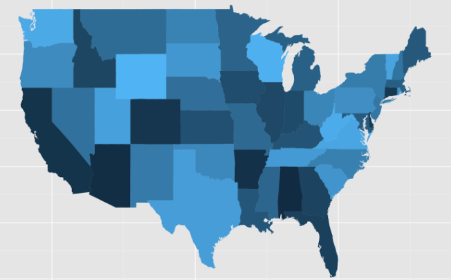
With this heat map, for example, we can see that not only do we have a ton of downloads in California, Colorado, and most of the south, we have weirdly few in Texas comparatively. Without a heat map visualizing this graphically, it can be difficult to recognize these spatial abnormalities.

When are our customers interacting? - Line Plot

We might also be interested in when customers downloaded our app. This can help us predict spikes in demand due to effects like seasonality.Whether it’s adjusting to external high volume days like Black Friday, or internal ones like  new product releases. Below is a sample of downloads for the first week of July, separated by Origin to see the different levels of 4 July spike in different countries.

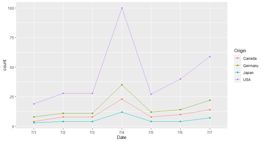
The vast, vast majority of our downloads in the 1st week of July were on July 4th. If we weren’t looking into plots like this, we might think our app is suddenly getting wildly popular and growing exponentially. In reality, this is likely an outlier day unlikely to happen again soon. Why might that be? As we saw earlier, the majority of our users are in the US, where July 4th is a notable hot dog eating occasion - which could lead to more users trying the app. Understanding outliers allows us to better predict how fast our app is actually growing, without baking in weird one off occurrences. It also lets us plan for another potential spike in usage the following July 4th.

How often are our customers interacting? - Histogram

We know where our customers are coming from and when they’re downloading, but how often are they using our app? It’s generally good practice to record data for when folks are using your product, and for Not Hotdog, that means knowing when users are opening the app and asking the age old question “Is this a hot dog?” For this, we might think of the amount of elapsed time between when returning users open our app, or cycle time. This helps us to predict usage in the future, while also knowing when to reach out to users that we would expect to have interacted again.

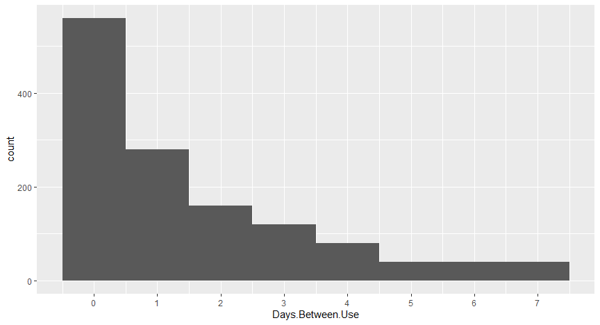
For our cycle time in days, we learn two things. First and foremost, many of our users are using multiple times on the same day. This is great news. They’re having successful first scans, and are coming back to scan again. The bad news is that once they’re done for the day, each day that passes makes them less likely to return. That means keeping users active is critical. For a closer look, we can look at our cycle in hours, or even filter to just users that use multiple times on the same day.

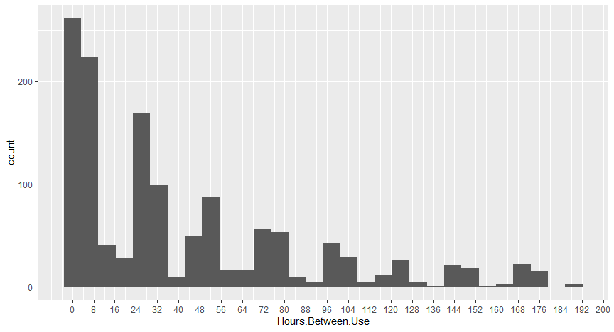
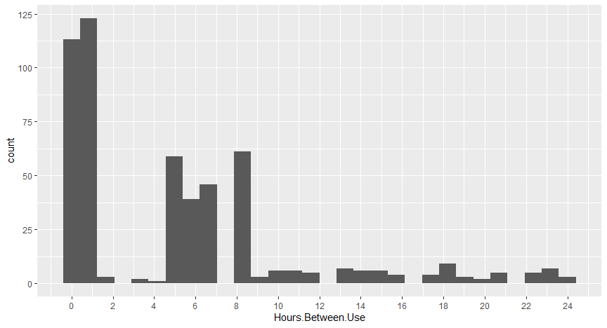
Most repeat uses are either immediately, scanning multiple items back to back, or are scanning roughly 5-6 hours later, which is also a good estimation of the gap between meal times when folks have food in front of them to scan. This is two different types of cycles depending on how fine grained we look into our data, both of which are popular types of cycles we might expect to find in data. With more data and more time, we might see that there are seasonal or yearly trends too.

Conclusion

Getting started visualizing data can feel intimidating, but it doesn’t have to be. There are many tools (including Datawisp) to help you do this and anyone can get started with just a little bit of effort. If your company has customers, and you have questions about how you can best leverage your data, don’t hesitate to reach out to us at hello@datawisp.io.